Filament2D Tutorial

This tutorial demonstrates the usage of the FilFinder2D object to perform the analysis on an individual filament. The general tutorial for FilFinder can be found here.

%matplotlib inline
import matplotlib.pyplot as plt
import astropy.units as u

# Optional settings for the plots. Comment out if needed.
import seaborn as sb
sb.set_context('poster')

import matplotlib as mpl
mpl.rcParams['figure.figsize'] = (12., 9.6)

The general tutorial demonstrates how the Filament2D objects interact with FilFinder2D. To generate an example, we will use a straight Gaussian filament to demonstrate how the FilFinder analysis can be run on individual filaments. We can also create a simplified mask by simply thresholding the image.

from fil_finder import FilFinder2D, Filament2D
from fil_finder.tests.testing_utils import generate_filament_model

mod = generate_filament_model(return_hdu=True, pad_size=30, shape=150,
                                  width=10., background=0.1)[0]

# Create a simple filament mask
mask = mod.data > 0.5

plt.imshow(mod.data, origin='lower')
plt.colorbar()
plt.contour(mask, colors='c', linestyles='--')

<matplotlib.contour.QuadContourSet at 0x7f1578dea630>

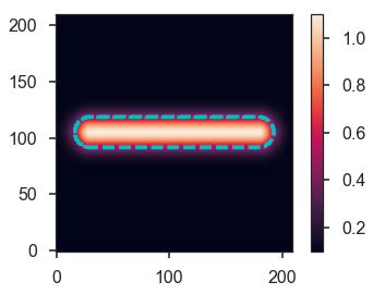
The simple filament model is shown above, with the mask highlighted by the dashed contour.

The first step is to run the first few steps on the FilFinder algorithm with FilFinder2D:

filfind = FilFinder2D(mod, distance=250 * u.pc, mask=mask)
filfind.preprocess_image(flatten_percent=85)

filfind.create_mask(border_masking=True, verbose=False,
                    use_existing_mask=True)
filfind.medskel(verbose=False)
filfind.analyze_skeletons()

/home/eric/Dropbox/code_development/filaments/build/lib.linux-x86_64-3.6/fil_finder/filfinder2D.py:288: UserWarning: Using inputted mask. Skipping creation of anew mask.
  warnings.warn("Using inputted mask. Skipping creation of a"

The Filament2D objects are created when running FilFinder2D.analyze_skeleton. From here, we will focus on the filament object:

fil = filfind.filaments[0]

The Filament2D object contains a minimized version of the FilFinder algorithm. Most of the FilFinder2D functionality simply loops throught the Filament2D objects. However, Filament2D object do not keep a copy of the data and are designed to carry a minimal amount of information.

Though not shown here, the only requirement to create a Filament2D object is a set of pixels that define the skeleton shape. These are contained in:

fil.pixel_coords

(array([105, 105, 105, 105, 105, 105, 105, 105, 105, 105, 105, 105, 105,
        105, 105, 105, 105, 105, 105, 105, 105, 105, 105, 105, 105, 105,
        105, 105, 105, 105, 105, 105, 105, 105, 105, 105, 105, 105, 105,
        105, 105, 105, 105, 105, 105, 105, 105, 105, 105, 105, 105, 105,
        105, 105, 105, 105, 105, 105, 105, 105, 105, 105, 105, 105, 105,
        105, 105, 105, 105, 105, 105, 105, 105, 105, 105, 105, 105, 105,
        105, 105, 105, 105, 105, 105, 105, 105, 105, 105, 105, 105, 105,
        105, 105, 105, 105, 105, 105, 105, 105, 105, 105, 105, 105, 105,
        105, 105, 105, 105, 105, 105, 105, 105, 105, 105, 105, 105, 105,
        105, 105, 105, 105, 105, 105, 105, 105, 105, 105, 105, 105, 105,
        105, 105, 105, 105, 105, 105, 105, 105, 105, 105, 105, 105, 105,
        105, 105, 105, 105, 105, 105, 105]),
 array([ 30,  31,  32,  33,  34,  35,  36,  37,  38,  39,  40,  41,  42,
         43,  44,  45,  46,  47,  48,  49,  50,  51,  52,  53,  54,  55,
         56,  57,  58,  59,  60,  61,  62,  63,  64,  65,  66,  67,  68,
         69,  70,  71,  72,  73,  74,  75,  76,  77,  78,  79,  80,  81,
         82,  83,  84,  85,  86,  87,  88,  89,  90,  91,  92,  93,  94,
         95,  96,  97,  98,  99, 100, 101, 102, 103, 104, 105, 106, 107,
        108, 109, 110, 111, 112, 113, 114, 115, 116, 117, 118, 119, 120,
        121, 122, 123, 124, 125, 126, 127, 128, 129, 130, 131, 132, 133,
        134, 135, 136, 137, 138, 139, 140, 141, 142, 143, 144, 145, 146,
        147, 148, 149, 150, 151, 152, 153, 154, 155, 156, 157, 158, 159,
        160, 161, 162, 163, 164, 165, 166, 167, 168, 169, 170, 171, 172,
        173, 174, 175, 176, 177, 178, 179]))

These pixel coordinates are the positions in the original image. When the skeleton array is generated, the minimal shape is returned:

plt.imshow(fil.skeleton())

<matplotlib.image.AxesImage at 0x7f157c3b3a90>

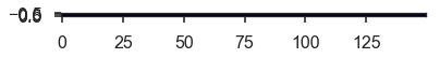
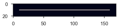
For a straight skeleton in this case, this returns a 1-pixel wide array in 0th dimension. This array can be padded:

plt.imshow(fil.skeleton(pad_size=10))

<matplotlib.image.AxesImage at 0x7f157bbefc50>

The position of the filament is defined as the median pixel location based on the set of skeleton pixels:

fil.position()

[<Quantity 105. pix>, <Quantity 104.5 pix>]

If WCS information is given for the object, the centre can also be returned in world coordinates:

fil.position(world_coord=True)

[<Quantity 359.99770817 deg>, <Quantity 0.00114592 deg>]

The skeleton analysis, equivalent to FilFinder2D.analyze_skeletons is Filament2D.skeleton_analysis. However, there are additional arguments that must be passed since the Filament2D object does not contain a copy of the image. To reproduce the fil.analyze_skeletons call from above, we can run:

fil.skeleton_analysis(filfind.image, verbose=True)

The same keyword and plot output is shown as described in the FilFinder2D tutorial.

The networkx graph can be accessed from fil.graph and can be plotted:

fil.plot_graph()

Filaments with multiple branches have more interesting looking graphs.

The lengths and branch properties are now defined:

fil.length()

\[149 \; \mathrm{pix}\]

fil.branch_properties.keys()

dict_keys(['length', 'intensity', 'number', 'pixels'])

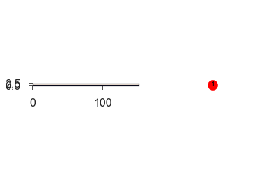
The longest path skeleton is now defined as well. The skeleton array of the longest path can be returned with:

plt.imshow(fil.skeleton(out_type='longpath', pad_size=10), origin='lower')

<matplotlib.image.AxesImage at 0x7f157be82518>

Orientation and Curvature

The RHT analysis on the longest path is run with:

fil.rht_analysis()
print(fil.orientation, fil.curvature)

1.5707963267948966 rad 0.26411662612097775 rad

The RHT distribution can be plotted with:

fil.plot_rht_distrib()

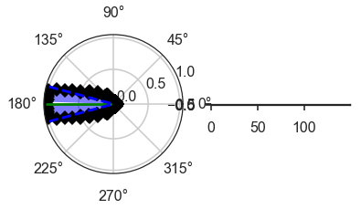
And the distribution can be accessed with Filament2D.orientation_hist, which contains the bins and the distribution values.

To run on individual branches, use:

fil.rht_branch_analysis()
print(fil.orientation_branches, fil.curvature_branches)

[1.57079633] rad [0.26411663] rad

The properties of branches can be returned with:

fil.branch_table()

Table length=1

length	intensity
pix
float64	float64
149.0	1.0999999999999996

And with the orientation and curvature branch information:

fil.branch_table(include_rht=True)

Table length=1

length	intensity	orientation	curvature
pix		rad	rad
float64	float64	float64	float64
149.0	1.0999999999999996	1.5707963267948966	0.26411662612097775

Radial Profiles and Widths

The radial profiles and width analysis is run with Filament2D.width_analysis. Most of the inputs are the same as those for FilFinder2D.find_widths, with a few key differences:

• The image must be given.

• The total skeleton array must also be given, since each Filament2D is unaware of other filaments.

• The beam width must be given for the FWHM to be deconvolved.

To reproduce the FilFinder2D analysis:

fil.width_analysis(filfind.image, all_skeleton_array=filfind.skeleton, beamwidth=filfind.beamwidth,
                   max_dist=0.3 * u.pc)

The radial profile is contained in fil.radprofile and can be plotted with:

fil.plot_radial_profile(xunit=u.pc)

The parameters, uncertainty, model type, and check for fit quality are contained in:

print(fil.radprof_parnames)
print(fil.radprof_params)
print(fil.radprof_errors)
print(fil.radprof_type)
print(fil.radprof_fit_fail_flag)

['amplitude_0', 'stddev_0', 'amplitude_1']
[<Quantity 1.00078556>, <Quantity 9.99775856>, <Quantity 0.09998652>]
[<Quantity 0.00189642>, <Quantity 0.0165278>, <Quantity 0.00059495>]
gaussian_bkg
False

The (possibly) deconvolved FWHM is:

fil.radprof_fwhm(u.pc)

(<Quantity 0.23351 pc>, <Quantity 0.0003924 pc>)

The first element is the FWHM and the second is the error.

Note that the fit has correctly recovered the model parameters set at the beginning.

An astropy table can be returned with the complete fit results:

fil.radprof_fit_table(unit=u.pc)

Table length=1

amplitude_0	amplitude_0_err	stddev_0	stddev_0_err	amplitude_1	amplitude_1_err	fwhm	fwhm_err	fail_flag	model_type
						pc	pc
float64	float64	float64	float64	float64	float64	float64	float64	bool	str12
1.0007855625803985	0.0018964160055463767	9.99775856017537	0.01652780418619165	0.09998652036316304	0.0005949451821499358	0.2335099973611502	0.00039239889215719536	False	gaussian_bkg

And finally the fit model itself can be accessed with:

fil.radprof_model

<CompoundModel3(amplitude_0=1.00078556, mean_0=0., stddev_0=9.99775856, amplitude_1=0.09998652)>

The radial profile can be returned as an astropy table with fil.radprof_table(xunit=u.pc).

Other Outputs

The total intensity of the filament within the FWHM is:

fil.total_intensity()

\[3497.8689 \; \mathrm{K}\]

And with the fitted background removed:

fil.total_intensity(bkg_subtract=True)

\[3112.3209 \; \mathrm{K}\]

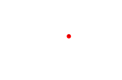
The model image from the radial profile fit:

plt.imshow(fil.model_image(), origin='lower')
plt.colorbar()

<matplotlib.colorbar.Colorbar at 0x7f157bd1ad68>

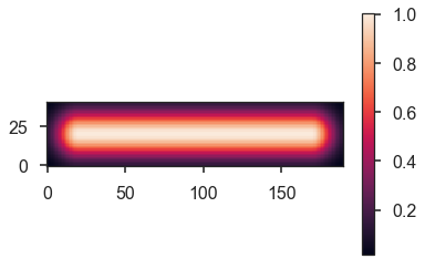
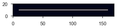
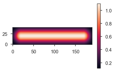
By default, the background level is subtraced. Without the subtraction:

plt.imshow(fil.model_image(bkg_subtract=False), origin='lower')
plt.colorbar()

<matplotlib.colorbar.Colorbar at 0x7f157b3434a8>

The median along the skeleton:

fil.median_brightness(filfind.image)

1.1

This is consistent with the max of the model image:

filfind.image.max()

\[1.1 \; \mathrm{K}\]

The profile along the longest path skeleton:

plt.plot(fil.ridge_profile(filfind.image))

[<matplotlib.lines.Line2D at 0x7f157bd30978>]

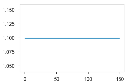
In this case, the ridge is constant in the model.

One feature that is not included in FilFinder2D is Filament2D.profile_analysis, which creates a set of profiles perpendicular to the longest path skeleton. This is useful for measuring filament properties as a function of position, rather than creating a single radial profile:

profs = fil.profile_analysis(filfind.image, xunit=u.pc, max_dist=30 * u.pix)
for dist, prof in zip(profs[0], profs[1]):
    plt.plot(dist, prof)
plt.ylabel("Amplitude")
plt.xlabel("Distance from skeleton (pc)")

Text(0.5,0,'Distance from skeleton (pc)')

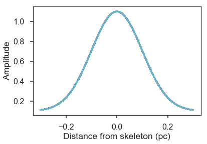
Plotted here are all of the radial profiles. For this model, however, they are all the same. Fitting of the radial profiles is not included in Filament2D due to the complexity that some radial slices can show in real filaments. See a dedicated package for this type of analysis, such as radfil.

Saving the Output

A FITS file can be saved with a stamp of the image, skeleton, longest path skeleton, and the filament model:

fil.save_fits("filament_stamp.fits", filfind.image)

Saving a Filament2D object

The object can be saved and loaded as a pickle file:

fil.to_pickle('filament.pkl')

loaded_fil = Filament2D.from_pickle('filament.pkl')
loaded_fil.length()

\[149 \; \mathrm{pix}\]